Tutorials - How to read NWB files / SSCx Portal

How to read NWB files tutorial

Introduction

NWB files can be read in the following ways:

Method 1: Read NWB files in Python with PyNWB (official tutorial)
Method 2: Read NWB files in Matlab with MatNWB (official tutorial)

Installation instructions for PyNWB

Install the latest version of Miniconda with Python 3.

Create an environment and install pynwb:

conda create --name nwb python=3
conda activate nwb
pip install pynwb==2

If you want to explore these tutorials install jupyter and matplotlib:
```
pip install jupyter matplotlib
jupyter notebook
```

Method 1: Read NWB files with PyNWB API

In [1]:

import numpy as np
from pynwb import NWBHDF5IO
import matplotlib.pyplot as plt

Import and define convenience functions.

In [2]:

from hdmf.common.hierarchicaltable import to_hierarchical_dataframe, flatten_column_index

def getNWBTimestamps(PatchClampSeries, absolute_time = False):
    '''Generate timestamps for any PatchClampSeries object.
    '''
    data_shape = PatchClampSeries.data.shape
    rate = PatchClampSeries.rate
    starting_time = PatchClampSeries.starting_time

    assert len(data_shape) == 1, 'Too many dimensions'
    if absolute_time == False:
        starting_time = 0.0
    nsamples = data_shape[0]
    timestamps = starting_time + np.linspace(0, nsamples/rate, nsamples)
    return timestamps

Load NWB file

In [3]:

filepath = '001_140709EXP_A1.nwb'

In [4]:

io = NWBHDF5IO(filepath, 'r', load_namespaces = True)
nwbfile = io.read()

Load all tables into memory

The easiest way to work with the data is to retrieve and combine all icephys tables in a single pandas DataFrame. This step can take some time.

For more details, please refer to the pynwb documentation.

In [5]:

# Consider using nwbfile.get_icephys_meta_parent_table() or nwbfile.icephys_experimental_conditions
# instead of nwbfile.icephys_repetitions
df = to_hierarchical_dataframe(nwbfile.icephys_repetitions).reset_index()
df = flatten_column_index(df, max_levels = 2)

Retrieve stimulus types

Stimulus types (also known as protocols, patterns, sequential recordings, or just stimuli) are stored in a dedicated column (stimulus_type) in the sequential_recordings table.

In [6]:

stimulus_types = sorted(df[('sequential_recordings','stimulus_type')].unique().tolist())

In [7]:

print(stimulus_types)

['APWaveform', 'DeHyperPol', 'Delta', 'ElecCal', 'FirePattern', 'HyperDePol', 'IDRest', 'IDThres', 'IV', 'NegCheops', 'PosCheops', 'RPip', 'RSealClose', 'RSealOpen', 'Rac', 'ResetITC', 'SetAmpl', 'SetISI', 'SineSpec', 'SponHold3', 'SponHold30', 'SponNoHold30', 'StartHold', 'StartNoHold', 'TestAmpl', 'TestRheo', 'sAHP']

Plot one stimulus-response pair

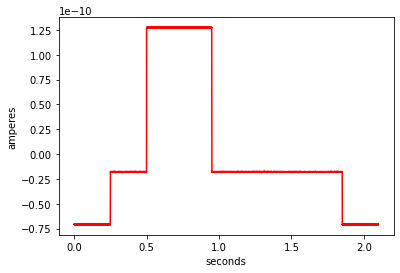
In [8]:

# Get stimulus and response traces
trace_no = 60
S = df[('stimuli','stimulus')][trace_no][2] # "2" refers to an implementation detail
R = df[('responses','response')][trace_no][2]

In [9]:

# Plot stimulus
plt.plot(getNWBTimestamps(S), S.data[:] * S.conversion,'r')
plt.xlabel('seconds')
_ = plt.ylabel(S.unit)

In [10]:

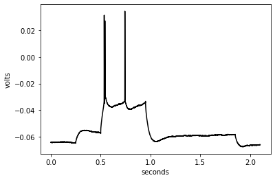
# Plot response
plt.plot(getNWBTimestamps(S), R.data[:] * R.conversion,'k')
plt.xlabel('seconds')
_ = plt.ylabel(R.unit)

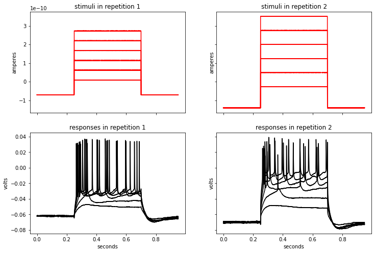
Retrieve and plot all traces of a given stimulus type (i.e. repetitions)

Choose one stimulus type from the list printed above.

In [11]:

st = stimulus_types[0]

In [12]:

df_st = df[df[('sequential_recordings','stimulus_type')] == st]
repetitions = df_st[('repetitions','id')].unique().tolist()

print(f'Stimulus {st}, repetitions {repetitions}')

Stimulus APWaveform, repetitions [1, 2]

Plot traces for each repetition.

(Please note that in the code below it is assumed that for each stimulus there is a response, and vice versa. The tuple (start_index, index_count, PatchClampSeries)will only contain None's if a trace does not exist.)

In [13]:

fig, axs = plt.subplots(2, len(repetitions), figsize = (12,8), sharex = 'col', sharey = 'row', squeeze = False)

for idx, rep in enumerate(repetitions):

    df_st_rep = df[(df[('sequential_recordings','stimulus_type')] == st) &
                   (df[('repetitions','id')] == rep)]
    stimuli = df_st_rep[('stimuli','stimulus')]
    responses = df_st_rep[('responses','response')]

    # S and R below are tuples: (start_index, index_count, PatchClampSeries)
    for S in stimuli:
        axs[0, idx].plot(getNWBTimestamps(S[2]), S[2].data[:] * S[2].conversion,'r')
        axs[0, idx].set_ylabel(S[2].unit)
        axs[0, idx].set_title(f'stimuli in repetition {idx+1}')

    for R in responses:
        axs[1, idx].plot(getNWBTimestamps(R[2]), R[2].data[:] * R[2].conversion,'k')
        axs[1, idx].set_ylabel(R[2].unit)
        axs[1, idx].set_title(f'responses in repetition {idx+1}')
        axs[1, idx].set_xlabel('seconds')

Method 2: Read NWB files in Matlab

Installation instructions

First download MatNWB. In a terminal type:

git clone https://github.com/NeurodataWithoutBorders/matnwb.git

This script has been tested on the commit 276e462 implementing NWB schema v2.4.0, so you might want to check out to it:

cd matnwb
git checkout 276e462

In Matlab, add the matnwb folder and its subfolders to Path and generate the core classes:

cd matnwb
addpath(genpath(pwd));
generateCore()

Then you can run this script.

For the full documentation visit https://github.com/NeurodataWithoutBorders/matnwb#matnwb.

Read NWB file

filename = '001_140709EXP_A1.nwb';

% Read file.
nwb = nwbRead(filename);